As a complex valued function of a complex variable, the graph of the Riemann zeta function ζ(s) lives in four dimensional real space. To get an idea of what the function looks like, we must do something clever.
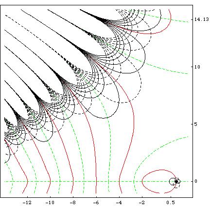
The real and imaginary parts of ζ(s) are each real valued functions; we can think of the graphs of each one as a surface in three dimensional space. Rather than look at two surfaces simultaneously, we can view the level curves for the two surfaces. The level curves are curves in the s plane showing points of constant height on the surface, as on a contour map.
Level curves for Re(ζ(s)) are shown above with the solid lines; the red curve is Re(ζ(s))=0, the black curves represent values other than zero. Level curves for Im(ζ(s)) are shown above with dotted lines; the green curve is Im(ζ(s))=0, the black curves represent values other than zero. The function ζ(s) is real on the real axis, thus Im(ζ(s))=0 there. Zeros of ζ(s) are points in the plane where both Re(ζ(s))=0 and Im(ζ(s))=0; these are points where the red and green curves cross. You can see the trivial zeros at the negative even integers, and the first nontrivial zero at s=1/2+i*14.135..., this is the point in the plane (1/2, 14.135...). You can also see the pole at s=1.
Another possibility is to view the complex number w=ζ(s), itself a point in the plane, as a vector in polar coordinates. The angle, or argument of ζ(s) is a number between 0 and 2π for each complex s. We can interpret this angle as a color on the color wheel, and plot a pixel with that color at the corresponding point in the domain, that it, in the s plane. In this representation, a zero of ζ(s) is a point where all the colors come together; you can see both trivial zeros and the first three non-trivial zeros. Each of these is a simple zero (as the Riemann Hypothesis predicts); going around the point once we see each of the colors exactly once. Observe the colors also come together at the pole s=1; but with a difference. At the pole one circles the color wheel in the opposite direction.
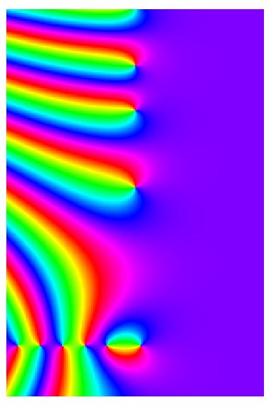
The Mathematica code which produced this is
Show[Graphics[RasterArray[Table[Hue[Mod[3Pi/2 +
	Arg[Zeta[sigma +I t]], 2Pi]/(2Pi)],
		 {t, -4.5, 30, .1}, {sigma, -11, 12, .1}]]],
			AspectRatio -> Automatic]
If we restrict the s variable to, say, a vertical line in the s plane, the values of w=ζ(s) will also be one dimensional, a curve in the w plane which we can plot. Changing the position of the vertical line makes the curve move. Each frame of the movie below shows a single such curve in the w plane, as the vertical line in the s plane moves from Re(s)=.05 to Re(s)=.95. The value of σ=Re(s) is shown at the top. Observe that the curves pass through the origin only in a single frame of the movie, when Re(s)=.5. This happens because all the low lying zeros of ζ(s) are known to satisfy the Riemann Hypothesis; they have real part equal to 1/2. In this movie we have colored each pixel again with the argument as above, but now we are looking at the range, not the domain, so colors are constant along rays emanating from the origin.
Alternately, we can fix σ=Re(s)=1/2, and make a movie where we trace out ζ(1/2+It) for increasing values of t. The value of t=Im(s) is shown at the top. The curve passes through the origin for each value of t such that ζ(1/2+It)=0, namely t = 14.135..., 21.022..., 25.011..., 30.425..., 32.935..., 37.586...
The reason for making the movies in color (aside from the fact that it is pretty) is that you see the color changes continuously, except when the curve passes through the origin, that is, when ζ(s)=0. The angle at which the curve exits the origin differs by a factor of π from the angle at which it entered the origin. We can use this to get a quick-and-dirty way to see that the prime numbers p determine the location of the zeros ρ of ζ(s). The argument of ζ(s) is the imaginary part of the logarithm log(ζ(s)). Borrowing an idea from the physicist Michael Berry, we take the logarithm of the Euler product over primes for ζ(s) at s=1/2+It, even though the product does not converge there. This gives a sum over primes p of terms -log(1-p^{1/2+It}), each of which can in turn be expanded using the series for log(1-z). Taking imaginary parts to get the argument, we have
arg(ζ(1/2+It)) "=" -Σ_p &Sigma_m sin(tmlog(p))/(mp^{m/2}).
The notation "=" is to remind you that the equality is only formal, the series does not converge. None the less, the first few terms are enough to indicate the rough location of the first few zeros. Below is shown the graph (in red) of arg(ζ(1/2+It)) on the vertical axis for t between 0 and 30 on the horizontal axis. The discontinuities at t = 14.135..., 21.022..., 25.011... show the location of the first three zeros. The movie shows (in black) the contribution of all powers of primes below 200 in the divergent series above, with one term added in each frame. Since the finite sum is a continuous function, there are no actual discontinuities, but it does the best it can.
(There is a famous quotation of the mathematicain George F. Carrier, who said "Divergent series converge faster than convergent series, because they don't have to converge." This movie is an example.)
The next section shows the converse idea, that is, how the zeros of the Riemann zeta function determine the location of the primes.
Next: Chapter 10 Explicit Formula