Progress Report
we have successfully written the sequential codes for adaptive Runge-Kutta 4-3 and Runge-Kutta 5-2. All codes were initially written in Matlab and then translated into C++. A separate folder holds DRWave.cpp which stores all the information about the Dieterich Ruina wave equation, which, after the method of lines, becomes a system of coupled nonlinear ODEs. The main function here defines the internal parameters for the DR ODEs and its initial data, then calls the desired Runge-Kutta method. So far we have experienced high computational time due to the small time step necessary to maintain accuracy. Some parameter combinations increase the intensity of the nonlinear terms, forcing us to take smaller time steps at the velocity approaches -1.
There are three general areas where we can parallelize this code and hopefully decrease computational time. The first is in the RK method’s matrix vector multiplication; the second is the RK method itself (pipelining the K's) and also time splitting (but since we don't know the solution at later times we can't do this). Our matrix vector multiplication will actually be much simpler than implementing a parallel matrix vector multiplication. If we distribute each u, v and theta vectors evenly across the processors, at each function evaluation, each processor need only MPI_send and MPI_Recv their boundary points. And if there is a sufficient number of "inner" points to compute we can hide the communication cost going on between neighboring processors. We can even experiment with various layers of ghost cells.
We have attempted to write C++ codes for the Adams-Bashford methods, but this as well as the constant coefficient Adams Bashorth-Moulton Predictor Corrector methods are not well suited for this particular problem. They do not have as strong stability properties as RK, the stiffness of the problem may be affecting the Adams methods more.
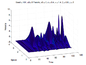
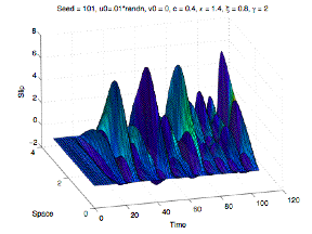
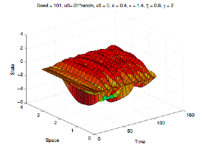
The plots below show the numerical solution (from sequential Matlab code) using the RK 4-3 method. The slip (u) is on the left, the slip velocity (v) in the middle, and the state variable (theta) is on the right. For this particular set of parameters, the solution appears chaotic in both time and space.